Progressive GAN Implementation

Link (code): https://github.com/altairmn/progressive-gan

Paper: https://arxiv.org/abs/1710.10196

Overview

Progressive GANs work by gradually adding layers to the discriminator and generator of the GAN during training. The benefits of this approach include faster training, reduced amortized memory and GPU usage over the course of training, and qualitatively better results. This paper is focused on training a GAN for generating from the distribution of CelebA-HQ dataset.

Notable Points

• Loss function is the wasserstein loss. Generator outputs an image from the toRGB layer, and the discriminator takes in an image in the fromRGB layer. toRGB layers: \(n \to 3\) channels, fromRGB layers: \(3 \to n\) channels.

• Generator Input input samples are from a 512 dimensional hyper sphere. So to sample for the generator, take a 512-dim random sample, and then normalize it to norm = 1

• Initialization: All weights in the network are initialized using a (0,1) normal distribution and bias with 0

• LCN (Local Response Norm) is used in the generator after every Conv layer. LCN normalizes each pixel slice across channels, and normalization constant is square root of average sum of squares. More on LCN

  nn.LocalResponseNorm(size = 2 * self.channel_dims[self.progress], alpha = 2, beta = 0.5, k = 1e-8)

• Minibatch standard deviation layer: after the last layer of the discriminator, there is a minibatch standard deviation layer. it computes the standard deviation for each feature in each spatial location across a minibatch. Then all these values are averaged to arrive at a single value. Then this value is replicated to create an extra channel (making channels go from \(512 \to 513\)) and concatenated to the input to the discriminator output layer.

def stddev(self, x):
    """
    Compute stddev
    """
    y = torch.sqrt(x.square().mean(dim=0) - x.mean(dim=0).square())
    return torch.mean(y)

• Equalized Learning Rate: This is the most tricky part of the paper. The weights in the generator are scaled at runtime i.e. after each learning step, you’d rescale the weights in the network. Each weight is set as \(w_i = w_i/c\) where \(c\) is the constant from He’s initializer. In this implementation, we use apply_elr method to scale the weights after each cycle of training.

def apply_elr(self):
    for param in self.named_parameters():
        if "weight" in param[0]:
            param[1].data = param[1].data * getHeMultiplier(param[1].data)

• Transition: When adding a new layer to the discriminator and generator, there’s an interim transition period to ensure that we don’t start out cold with the new layers’ weights. Transition for discriminator and generator is described here.

Architecture

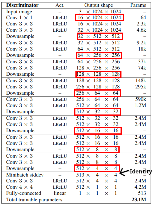
The boxed sizes are the outputs of the fromRGB layers.

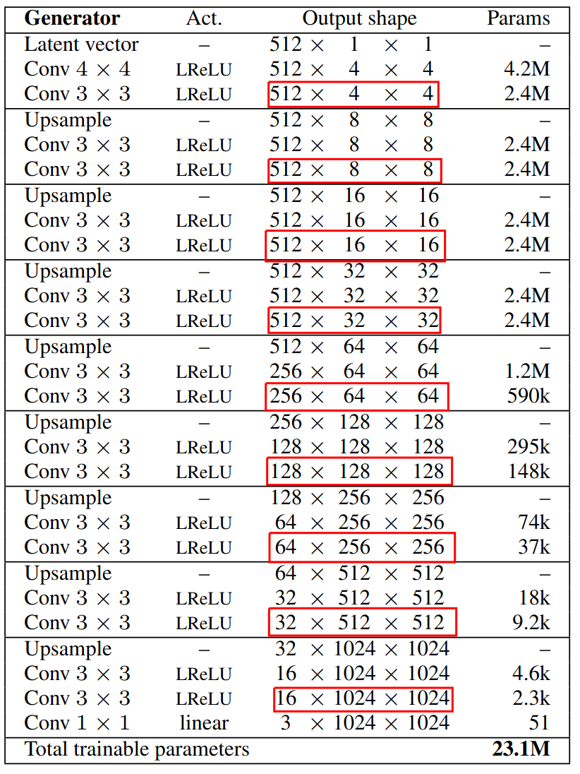
The boxed represent the input sizes to the toRGB layer

Transition

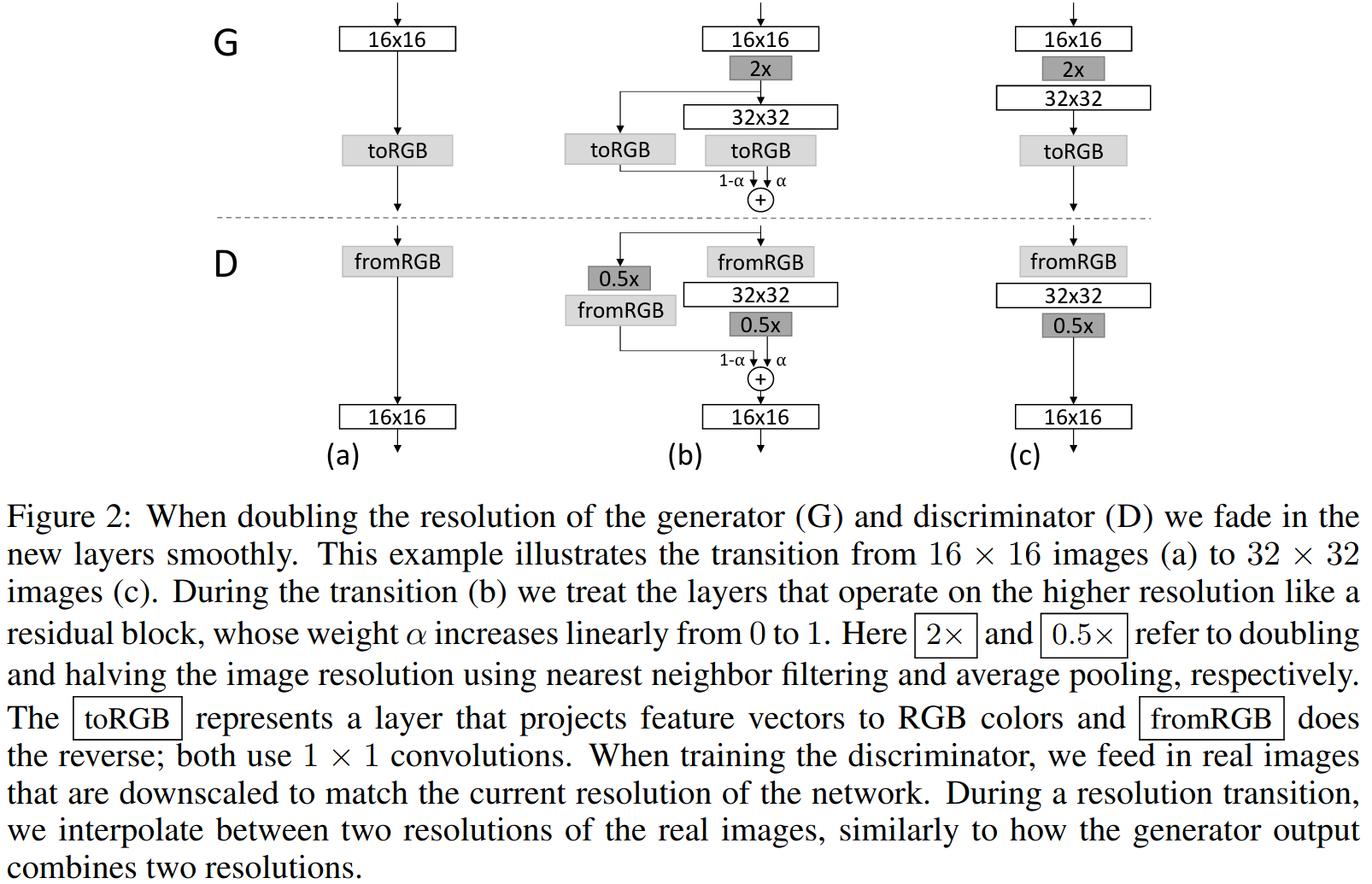
Each transition is two step:

• (b) Add new layers, and setup a new input/output layer depending on discriminator or generator
• (c) Discard the old input/output layers i.e. fromRGB and toRGB layers

To achieve this, this implementation uses the alpha value as an indicator of the step (b) or (c).

Transition in Generator

def transition(self):
    if self.alpha == 0.0:
        self.progress = self.progress + 1
        self.alpha = 0.5
        self.inputs.insert(0, nn.Conv2d(in_channels=3,out_channels=self.channel_dims[self.progress],kernel_size=1))
        self.layers.insert(0, nn.Sequential(
            nn.Conv2d(in_channels=self.channel_dims[self.progress],out_channels=self.channel_dims[self.progress],kernel_size=3,padding=1),
            nn.LeakyReLU(0.2),
            nn.Conv2d(in_channels=self.channel_dims[self.progress],out_channels=self.channel_dims[self.progress-1],kernel_size=3,padding=1),
            nn.LeakyReLU(0.2),
            nn.AvgPool2d(kernel_size=2,stride=2)))
        print("Adding transition layers")
        else:
            self.alpha = 0.0
            print("Completing transition")
            return self.progress

Transition in Discriminator

def transition(self):
    if self.alpha == 0:
        self.progress = self.progress + 1
        self.alpha = 0.5
        self.outputs.append(nn.Conv2d(self.channel_dims[self.progress],3,kernel_size=1))
        self.layers.append(nn.Sequential(
            nn.Upsample(scale_factor = 2, mode = 'nearest'),
            nn.Conv2d(in_channels=self.channel_dims[self.progress-1],out_channels=self.channel_dims[self.progress],kernel_size=3,padding=1),
            nn.LocalResponseNorm(size = 2 * self.channel_dims[self.progress], alpha = 2, beta = 0.5, k = 1e-8),
            nn.LeakyReLU(negative_slope = 0.2),
            nn.Conv2d(in_channels=self.channel_dims[self.progress],out_channels=self.channel_dims[self.progress],kernel_size=3,padding=1),
            nn.LocalResponseNorm(size = 2 * self.channel_dims[self.progress], alpha = 2, beta = 0.5, k = 1e-8),
            nn.LeakyReLU(negative_slope = 0.2)
        ))
        else:
            self.alpha = 0

Note how alpha value is toggled. The progress instance variable is useful to get the appropriate values of the dimensions for that stage of training.

❗ This implementation also uses an identity layer as a hidden layer to start for clean code. You can see it marked in the Discriminator architecture diagram.

Use of Local Response Norm

To control the magnitudes in the generator, LRN is employed. It normalizes each pixel \(a_{x,y}\) in the activation that the sum of \(N\) neighboring pixels across channels is 1. This is done like so: \[ b_{x,y} = a_{x,y}/\sqrt{\sum_{j=0}^{N-1} (a_{x,y}^j)^2 + \epsilon} \quad {\epsilon>0, <<<1} \]

Pytorch computes it in this way: \[ b_{c} = a_{c}\left(k + \frac{\alpha}{n} \sum_{c'=\max(0, c-n/2)}^{\min(N-1,c+n/2)}a_{c'}^2\right)^{-\beta} \] In this network, the whole vector across channels is normalized, so the layer is specified as

nn.LocalResponseNorm(size = 2*n, alpha = 2, beta = 0.5, k = 1e-8) # n is number of channels

we normalize the feature vector in each pixel to unit length in the generator after each convolutional layer.

In this implementation, we apply the normalization after the leaky ReLU layer, and not before.