Implementing StarGAN

Paper: StarGAN: Unified Generative Adversarial Networks for Multi-Domain Image-to-Image Translation

Introduction

Image-to-image translation refers to mapping images between different domains. For example, changing the facial expression of a person from smiling to frowning, or changing the gender of a person from male to female, or their hair color from black to brown.

For each domain (ex: black_hair_color, or beard) every image has a value. In the dataset that we use, the values are yes/no. Of course, it’s possible that these domains or aspects of images don’t vary independently in naturally occuring examples. But that’s what makes some of the results interesting 😄.

StarGAN¹ performs this image-to-image translation task for face images. Before StarGAN, to learn mappings between 4 domains, we’d need 12 networks. Why? Let A, B, C and D be the domains. Then we have

$$\begin{aligned} I_A &\xrightarrow{G_1} I_B \\ I_A &\xrightarrow{G_2} I_C \\ I_A &\xrightarrow{G_3} I_D \\ &\ldots \\ I_D &\xrightarrow{G_{10}} I_A \\ I_D &\xrightarrow{G_{11}} I_B \\ I_D &\xrightarrow{G_{12}} I_C \end{aligned}$$

where $I_A\in A, I_B \in B \ldots$ are images in their respective domains. As you can see we’d need $G_1 \ldots G_{12}$ to perform the translations.

StarGAN learns to map between multiple domains by using a single network. Roughly, it achieves this by passing in domain information to the network: $$\begin{aligned} I_A,F_B &\xrightarrow{G} I_B \\ I_C,F_D &\xrightarrow{G} I_D \\ \end{aligned}$$ where $F_B$ and $F_D$ encode information of output domain.

Datasets

CelebA: ~200K RGB face images of celebrities. each has 40 attributes. size of images is 178x218. Each attribute is $\{0,1\}$ such as Brown_Hair, Young, Big_Nose, etc.

The preprocessing pipeline for the images is:

The green blocks are augmentation blocks, and red blocks are transformation blocks.

Principal

The idea is to have a generator take in a source image $I$, and a $\{0,1\}$ attribute vector $\vec{l}$ which describes the target domain. The generator output $I_o$ is then fed into a classifier that checks if $I_o$ can be classified as $\vec{l}$. An additional objective ensures that the difference between $I$ and $I_o$ is minimized so that the images look similar (imagine same person with different hair color for example).

Before we delve into StarGANs details, a brief introduction to GAN (Generative Adversarial Networks) is given below.

Overview of GANs

Generative Models

Generative adversarial networks are an example of generative models ²

A generative model takes a dataset consisting of samples drawn from a training set $p_{data}$ and learns to represent and estimate of that distribution somehow. The result is the probability distribution $p_{model}$.

Among the many reasons for studying generative models, one that I find most motivating is the ability of generative models to work with multi-modal outputs i.e. there are many correct answers to a possible question (Ex: “generate image of a dolphin” can generate a lot of different variants). However, if we use MSE, for instance, the output will be the average of all correct answers which is not always desired.

From the maximum likelihood lens, the objective of a generative model is to find parameters $\theta$ that maximize the likelihood of the training data $x^{(i)}$ where $i \in \{1, \ldots, m\}$ which means there are $m$ examples in the training set. $$\theta^* = \arg\max_\theta{\sum_{i=1}^m\log p_{model}(x^{(i)};\theta)}$$ Equivalently $$\theta^* = \arg\max_\theta{\mathbb{E}_{x\sim p_{data}}\log p_{model}(x;\theta)}$$

In explicit models, you explicitly write down the likelihood of the data under $p_{model}$. However, maximizing it is another challenge since gradient-based methods may not be computationally tractable in all cases.

In implicit models, you can only sample from the estimated density, not express the density itself i.e. you can only interact with $p_{model}$ by sampling from it. GANs are an example of implicit models.

Summary of GAN

The generator $G$ in a GAN transforms a random variable $Z$ to $X$ which is in the space we care about. Therefore, $G$ gives us a way to sample from $p_{model}$. But how do we tune the parameters $\theta$ of distribution $G(Z)$ so that we can increase the likelihood? Well, we can do it by evidence.

One way is to judge if the samples from $p_{model}$ are indistinguishable from samples from $p_{data}$.The hypothesis is that if this is done for enough samples, then we can make an accurate judgement about $p_{model}$ i.e. be able to tell if $p_{model}$ is close to $p_{data}$ or not.

To make this judgement, we use a discriminator $D$. The discriminator is taught to recognize whether a sample is from $p_{data}$ or not. If the discriminator can recognize this perfectly, then in theory $G$ can tune it’s parameters $\theta$ until $D$ evaluates all outputs of $G$ (i.e. $p_{model}$) to be sampled from $p_{data}$ as well.

GAN Loss Function

For a GAN discriminator $D$, we use the standard cross-entropy cost: $$J^{(D)}(\theta,\phi) = -\frac{1}{2}\mathbb{E}_{x\sim p_{data}}\log(D(x)) -\frac{1}{2} \mathbb{E}_{z}\log(1-D(G(z)))$$ There are multiple choice of losses for the generator $G$. One is $J^{(G)}=-J^{(D)}$ i.e. try to maximize discriminator loss which would mean that discriminator will classify generator outputs.

From the standpoint of ensuring that both discriminator and generator have strong gradients when they’re “wrong”, we change the functions up a bit; however, these are heuristics.

Note: As a standard, for $D$ label $0$ means fake, and label $1$ means real. So for all generated inputs, it must predict $0$.

StarGAN Overview

Output

Generator

The basic generator architecture is as follows:

Discriminator

The discriminator architecture:

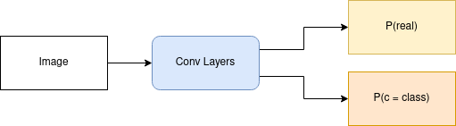
According to the paper, the discriminator leverages PatchGANs

which classify whether local image patches are real or fake.

However, in the network described in the appendix, the output $D_{src}$ is not 1-dimensional. Instead it’s 2x2 for a 128x128 image. This is because the size of output is $\left(\frac{h}{64},\frac{w}{64},1\right)$.

In the PatchGAN architecture, in the last layer a convolution is applied to get a 1D output, followed by a Sigmoid function. Accordingly, we make the following modifications to the StarGAN architecture:

• Final Conv kernel_size=2, padding=0 to get 1D output
• Sigmoid applied to get output $\in [0,1]$

The other output of the discriminator is used to compute classification loss, which is described later.

Training Methodology

There are three losses in StarGAN and the Generator and Discriminator have different goals with regards to these functions

Adversarial Loss

$$L_{adv} = \underbrace{\mathbb{E}_x[\log D_{src}(x)]}_{\alpha} + \underbrace{\mathbb{E}_{x,c}[1-\log D_{src}(G(x,c))]}_{\beta}$$ It helps to think here that $D_{src}(x) = P(\text{real}|x)$ i.e. probability that the source of $x$ is real or fake.

$D$ wants to maximize it’s ability to tell real and fake apart. So it wants that $P(\text{real}|x_{real}) \uparrow$ and $\left(P(\text{fake}|x_{fake}) = 1-P(\text{real}|x_{fake})\right)\uparrow$ i.e. $P(real|x_{fake})\downarrow$³

Which means, $D$ wants to maximize $L_{adv}$. On the other hand, $G$ wants to make sure that $D$ classifies generated images as real, therefore $G$ wants to maximize $P(real|x_{fake})$ i.e. minimize $\beta$ term which is effectively trying to minimize $L_{adv}$ since $G$ is only present in $\beta$.

In reality, StarGAN uses the Wasserstein GAN objective to stabilize training (more on WGAN loss in later posts 🔮) $$L_{adv}(D) = \underbrace{\mathbb{E}_x[D_{src}(x)]}_{\alpha} - \underbrace{\mathbb{E}_{x,c}[D_{src}(G(x,c))]}_{\beta} -\underbrace{\lambda_{gp}\mathbb{E}_{\hat{x}}\left[(\|\nabla_{\hat{x}}D_{src}(\hat{x})\|_2-1)^2\right]}_{\gamma}$$ where the $D$ wants $\alpha\uparrow$, $\beta \downarrow$, and $\gamma \downarrow$. If we take signs into account, then we find that $D$ wants to minimize $-L_{adv}(D)$. Also, here $\hat{x}$ is sampled from a straight line between fake and real images.

The adversarial loss for $G$ on the other hand is $$L_{adv}(G) = \underbrace{\mathbb{E}_{x,c}[D_{src}(G(x,c))]}_{\beta}$$ where $G$ wants $\beta \uparrow \implies -L_{adv}(G)\downarrow$

Classification Loss

Because we’re using a single $G$ network to generate images for all domains, we pass in target domain information say $F_A$ for domain $A$ to $G$ as well. For the generated image $I$, we want the discriminator to both think it’s real and classify it as $I\in A$.

Therefore, we have a classification loss as well. Since the labels in this task look like:

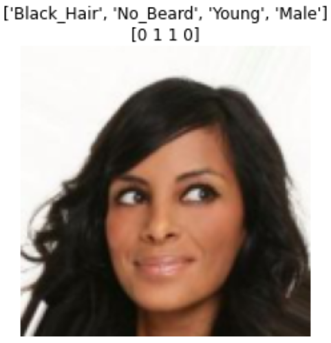
The classification for each image is multilabel multiclass. Therefore the loss is a sigmoid followed up binary cross entropy on each class $c^i_I$ for class vector $\vec{c}_I$ of image $I$:

$$L_{cls}(D) = \sum_{i} \text{BCELoss}(D(I)^i, c^i_I)$$ For generator $$L_{cls}(G) = \sum_i BCELoss(D(G(I,c))^i, c^i)$$ where $c$ is a class vector used to domain transfer image $I$ to labels $c$. In summary , $G$ wants to generate images that fool the discriminator, and that are classified in the correct class.

Reconstruction Loss

Lastly, we want to ensure that the only difference between $x$ and resulting $y$ is that of the domain. To handle this, we apply a cycle consistency loss i.e. transform image to class $c$, then transform output to class $c'$ which is class of $x$. $$L_{rec} = \mathbb{E}_{x,c,c'}[\|x - G(G(x,c),c')\|_1]$$ Note about Generator Training: When generator is being trained, random labels are fed in for images, instead of true labels. This means the generator may be asked to perform multiple domain translations at once. As to whether its better performance when a single domain translation is required, vs. multiple domain translations, that’s hard to tell. But it is assumed that the generator will eventually learn which entry in the domain vector correspond to what domain (i.e. for example $d[3] = 1$ => Black Hair)

Important things during training

• Pytorch optimizers minimize the loss since they subtract the gradient from the loss function $\implies$ pytorch performs gradient descent. Therefore, all objectives must be specified as min objectives.
• GAN training requires alternating between training the discriminator, and the generator. In StarGAN, there’s 1 iteration of training $G$ for every 5 iterations of training $D$.

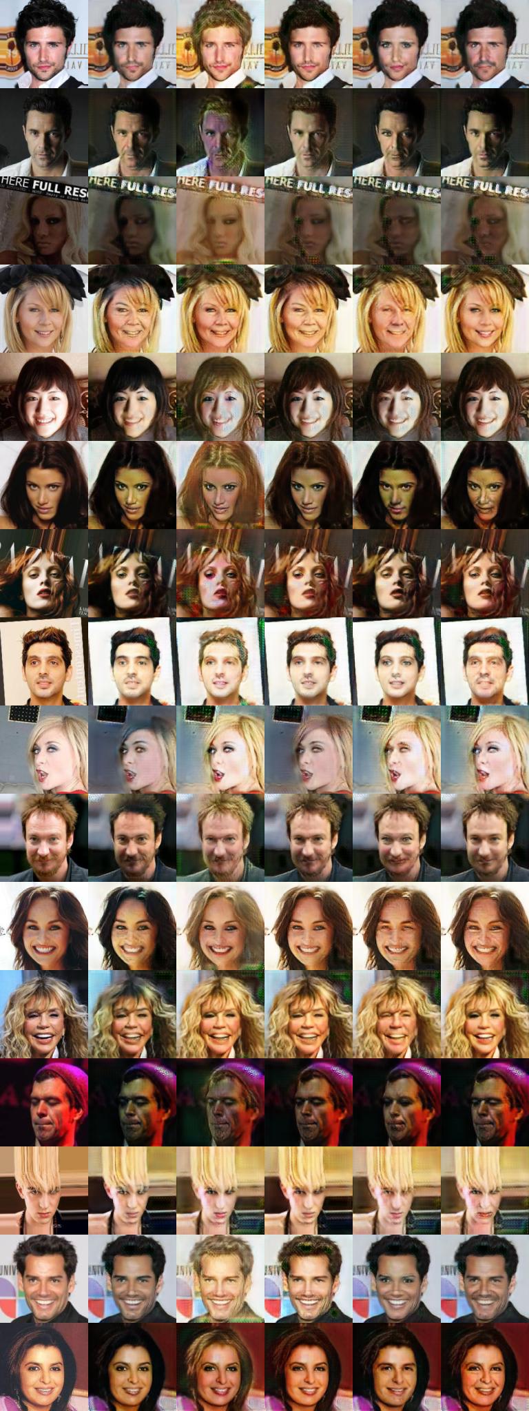
Results

We compare the results on the same sample of images earlier in the training vs. after 90K iterations. For each image, the samples are generated by flipping the value of 1 attribute.

In the training (and sampling), the selected attributes are:

[Black_Hair, Blond_Hair, Brown_Hair, Male, Young]

Caveat: Attributes associated with hair color are not flipped. Instead one of them is set to 1 while other hair color attributes are set to 0.

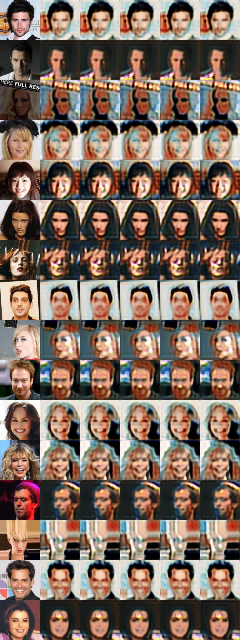
[Black_Hair, Blond_Hair, Brown_Hair, Male, Young]

Observe the changing hair colors, and changed face structure to reflect gender/age.

What’s wrong with StarGAN?

We randomly generate the target domain label so that $G$ learns to flexibly translate the input image.

This makes no sense. Assume there are 5 domains. Then the domain labels for that image are of the type $[d_1, d_2, d_3, d_4, d_5]$ where $d_i \in \{0,1\}$. If you feed in random labels for an image, then how does provide any hint to the generator? And if the purpose later on is to control for all domains except the one that is changed, then how will the generator learn for test time? Shouldn’t test conditions be the same as train conditions? Because during sampling/testing the label vector for the source image is preserved except the attribute that needs to be changed for ex: changing hair color.

FAQ

Generator Input

Class vector $\vec{c} \in \{0,1\}^n$ where $n$ is the number of classes. Then how is the label vector appended to the image to feed into the generator?

Consider image of size $4\times4$ and $n=2$ so the labels are changed like so:

array([1, 1])

array([[[1, 1, 1, 1],
        [1, 1, 1, 1],
        [1, 1, 1, 1],
        [1, 1, 1, 1]],

       [[1, 1, 1, 1],
        [1, 1, 1, 1],
        [1, 1, 1, 1],
        [1, 1, 1, 1]]])

After appending to a 3-channel image $3\times4\times4$ the final size is $5\times4\times4$. This is the input to the generator.

Logits

From the SO answer: https://stackoverflow.com/questions/41455101/what-is-the-meaning-of-the-word-logits-in-tensorflow

The raw predictions which come out of the last layer of the neural network.

1. This is the very tensor on which you apply the argmax function to get the predicted class.
2. This is the very tensor which you feed into the softmax function to get the probabilities for the predicted classes.

The logit seems to refer to real-valued tensor that is fed into some activation function to get the task output or before applying loss function to it. In case of classification, logit transforms real-valued tensor to probabilities.

This comes from the math definition of logit which refers to functions mapping probabilities $[0,1]$ to $[-\infty, +\infty]$. In context of NN, instead of the function(s), logit refers to the output of the function (which is to be fed into an activation function to get probabilities).

GPU Computation

As long as you make sure that all your leaf-nodes in the computation graphs are placed on the GPU, all operations will happen in the GPU.

Therefore, for every input tensor, place it on GPU by using .to(device)

Pytorch detach()

pytorch detach operation on tensors:

The only thing detach does is to return a new Tensor (it does not change the current one) that does not share the history of the original Tensor.

Why is x_fake.detach() is perfomed before passing the tensor to the discriminator? This is because we want to treat it as an ordinary input to the discriminator, and while training do not want to propagate the gradients back to the generator. While training the generator, we’ll push the gradients (at that time we should zero out the gradients of the discriminator).

Gradient Penalty

def gradient_penalty(y, x):
    """Compute gradient penalty: (L2_norm(dy/dx) - 1)**2."""
    weight = torch.ones(y.size()).to(self.device)
    dydx = torch.autograd.grad(outputs=y,
                               inputs=x,
                               grad_outputs=weight,
                               retain_graph=True,
                               create_graph=True,
                               only_inputs=True)[0]

    dydx = dydx.view(dydx.size(0), -1)
    dydx_l2norm = torch.sqrt(torch.sum(dydx**2, dim=1))
    return torch.mean((dydx_l2norm-1)**2)

Why is gradient penalty computed this way?

only_inputs=True because the input x is a mixture of generated fake images, and real images. When computing the gradient, we don’t want the gradient to propagate through the generator.

create_graph=True because y is discriminator output of x, and gradient penalty term is present in adversarial loss $L_{adv}$ for the discriminator. We want this term to be differentiable w.r.t. parameters of D i.e. we’ll be computing: $$\partial\left(\frac{\partial (\hat{x})}{\hat{x}}\right)/\partial \theta$$ create_graph indicates that we need the graph for the backward step. We don’t have retain_graph=True because we don’t need this graph after backward is called once. For different inputs, the graph is reconstructed (i.e. for each iteration of training there is a new graph).

References

The modified code can be found in the repository https://github.com/altairmn/stargan.